Data Release Overview
The data release consists primarily of images and catalogs. If you just want to browse the images, try the Navigator and cosmic wallpaper links at right. If you want the FITS files, proceed to the image access page. For catalogs, including photometric redshifts, proceed to the catalog access page. We also continue to maintain the archive of transients detected during observing. The rest of this page contains background info which may help you understand the data.
Coordinates: the DLS consists of five widely separated 2x2 degree fields with J2000 coordinates centered at:
| Field | RA | Dec | l,b | Ecliptic |
| F1 | 00:53:25.3 | +12:33:55 | 125,-50 | 17,6 |
| F2 | 09:19:32.4 | +30:00:00 | 197,44 | 133,14 |
| F3 | 05:20:00 | -49:00:00 | 255,-35 | 69,-72 |
| F4 | 10:52:00 | -05:00:00 | 257,47 | 166,-11 |
| F5 | 13:59:20 | -11:03:00 | 328,49 | 212,1 |
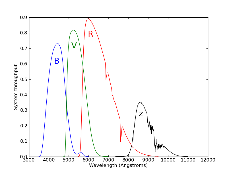
Filters: The throughput curves in each filter, as published in Schmidt & Thorman (2013), are available as ASCII files: B, V, R, and z. Note that the z curve as calibrated by thousands of stars in Schmidt & Thorman (2013) differs substantially from the NOAO version. Because the Johnson-Cousins BVR filters are calibrated by comparison to Landolt standards on the Vega system and the z filter was calibrated by overlap with SDSS, the BVR magnitudes are in the Vega system and the z magnitudes are in the AB system. If you wish to convert a z magnitude to the Vega system, subtract 0.549. To convert B, V, and R magnitudes to the AB system, add -0.105, 0.006, and 0.210 respectively.
Depth and masking: the depth is variable. If your science depends on having a uniform selection function, please take note of the THRESHOLDR field in the Sextractor table, which indicates the detection threshold (in ADU) at the position of each object. If you are working with images rather than catalogs, use the weight image (explained in the image access page) to determine relative depths. The weight image for a typical 40'x40' subfield looks like this:
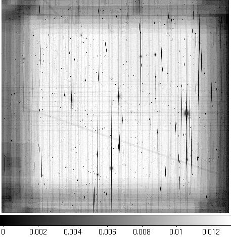
In addition to localized holes due to bright stars, satellite trails, etc, there are shallow areas around the edges. Each 2-degree-square field is composed of a 3x3 grid of these subfields. Averaging over these spatial variations, the depth as measured by recovery rate (as a function of R-band magnitude) of synthetic objects is plotted here:
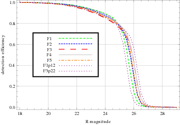
Each field is plotted here, as well as the deepest and shallowest individual subfields (the survey has 45 subfields). Masks which specify "bad" areas on the stacked images are described on the catalog access page.
Other details: R band consistently has the best seeing (<=0.9" vs 0.9-1.25" in BVR) and is the deepest, so our catalog uses R as the detection image. You can read more about the field selection, survey strategy, etc, in Wittman et al (2002). A paper with full details of the image stacking and catalog production is in preparation and will be linked to here when submitted.